RUSSIAN ACADEMY OF THE NATIONAL ECONOMY AND PUBLIC SERVICE UNDER THE PRESIDENT OF THE RUSSIAN FEDERATION
OREL BRANCH
Department of Mathematics and Mathematical Methods in Management
Independent work
Mathematics
on the topic "Variational series and its characteristics"
for full-time students of the Faculty of Economics and Management
areas of training "Personnel Management"
Objective: Mastering the concepts of mathematical statistics and methods of primary data processing.
An example of solving typical problems.
Task 1.
The following data was obtained by polling ():
1 2 3 2 2 4 3 3 5 1 0 2 4 3 2 2 3 3 1 3 2 4 2 4 3 3 3 2 0 6
3 3 1 1 2 3 1 4 3 1 7 4 3 4 2 3 2 3 3 1 4 3 1 4 5 3 4 2 4 5
3 6 4 1 3 2 4 1 3 1 0 0 4 6 4 7 4 1 3 5
Necessary:
1) Compile a variational series (statistical distribution of the sample), having previously recorded a ranked discrete series of options.
2) Construct a polygon of frequencies and a cumulate.
3) Compile a series of distributions of relative frequencies (frequencies).
4) Find the main numerical characteristics of the variation series (use simplified formulas to find them): a) arithmetic mean, b) median Me and fashion Mo, c) dispersion s2, d) standard deviation s, e) coefficient of variation V.
5) Explain the meaning of the results obtained.
Solution.
1) For compiling ranked discrete series of options sort the survey data by size and arrange them in ascending order
0 0 0 0 1 1 1 1 1 1 1 1 1 1 1 1 1 2 2 2 2 2 2 2 2 2 2 2 2 2 2
3 3 3 3 3 3 3 3 3 3 3 3 3 3 3 3 3 3 3 3 3 3 3 3 4 4 4 4 4 4 4 4 4 4 4 4 4 4 4 4
5 5 5 5 6 6 6 7 7.
Let's make a variation series by writing the observed values (options) in the first row of the table, and the frequencies corresponding to them in the second row (Table 1)
Table 1.
2) The frequency polygon is a broken line connecting the points ( x i; n i), i=1, 2,…, m, where m X.
Let's depict the range of frequencies of the variational series (Fig. 1).

Fig.1. Frequency polygon
The cumulative curve (cumulate) for a discrete variational series is a broken line connecting the points ( x i; n i nak), i=1, 2,…, m.
Let's find the accumulated frequencies n i nak(the cumulative frequency shows how many variants were observed with a trait value less than X). The found values are entered in the third row of table 1.
Let's build a cumulate (Fig. 2).

Fig.2. Cumulate
3) Find the relative frequencies (frequencies) , where , where m– number of different feature values X, which will be calculated with the same accuracy.
Let's write a series of distributions of relative frequencies (frequencies) in the form of table 2
table 2
4) Let's find the main numerical characteristics of the variational series:
a) We find the arithmetic mean using the simplified formula:
 ,
,
where - conditional options
Let's put With= 3 (one of the average observed values), k= 1 (difference between two adjacent options) and compile a calculation table (Table 3).
Table 3
| x i | n i | u i | u i n i | u i 2 n i |
| -3 | -12 | |||
| -2 | -26 | |||
| -1 | -14 | |||
| Sum | -11 |
Then the arithmetic mean

b) Median Me Variation series is the value of the feature that falls in the middle of the ranged series of observations. This discrete variational series contains an even number of terms ( n=80), so the median is equal to half the sum of the two median options.
Fashion Mo variation series is called the variant, which corresponds to the highest frequency. For a given variational series, the highest frequency n max = 24 corresponds to the variant X= 3 means fashion Mo=3.
c) dispersion s2, which is a measure of the dispersion of possible values of the indicator X around its average value, we find using the simplified formula:
 , where u i- conditional options
We will also enter intermediate calculations in Table 3.
Then the variance

d) Standard deviation s find by the formula:
![]() .
.
e) Coefficient of variation V: (),
The coefficient of variation is a dimensionless quantity, so it is suitable for comparing the scattering of variational series, the variants of which have different dimensions.
The coefficient of variation
![]() .
.
5) The meaning of the obtained results is that the value characterizes the average value of the feature X within the considered sample, that is, the average value was 2.86. Standard deviation s describes the absolute dispersion of the values of the indicator X and in this case is s≈ 1.55. The coefficient of variation V characterizes the relative variability of the indicator X, that is, the relative spread around its mean value, and in this case is .
Answer: ; ; ; .
Task 2.
We have the following data on the equity capital of the 40 largest banks in Central Russia:
| 12,0 | 49,4 | 22,4 | 39,3 | 90,5 | 15,2 | 75,0 | 73,0 | 62,3 | 25,2 |
| 70,4 | 50,3 | 72,0 | 71,6 | 43,7 | 68,3 | 28,3 | 44,9 | 86,6 | 61,0 |
| 41,0 | 70,9 | 27,3 | 22,9 | 88,6 | 42,5 | 41,9 | 55,0 | 56,9 | 68,1 |
| 120,8 | 52,4 | 42,0 | 119,3 | 49,6 | 110,6 | 54,5 | 99,3 | 111,5 | 26,1 |
Necessary:
1) Build an interval variation series.
2) Calculate the sample mean and sample variance
3) Find the standard deviation, and the coefficient of variation.
4) Construct a histogram of distribution frequencies.
Solution.
1) Let's choose an arbitrary number of intervals, for example, 8. Then the width of the interval:
![]() .
.
Let's make a calculation table:
| interval option, x k – x k +1 | Frequency, n i | Interval midpoint x i | conditional option, and i | and i n i | and i 2 n i | (and i + 1) 2 n i |
| 10 – 25 | 17,5 | – 3 | – 12 | |||
| 25 – 40 | 32,5 | – 2 | – 10 | |||
| 40 – 55 | 47,5 | – 1 | – 11 | |||
| 55 – 70 | 62,5 | |||||
| 70 – 85 | 77,5 | |||||
| 85 – 100 | 92,5 | |||||
| 100 – 115 | 107,5 | |||||
| 115 – 130 | 122,5 | |||||
| Sum | – 5 |
The value chosen as a false zero c= 62.5 (this option is located approximately in the middle of the variation series) .
Conditional options are determined by the formula
- introductory lesson is free;
- A large number of experienced teachers (native and Russian-speaking);
- Courses NOT for a specific period (month, six months, year), but for a specific number of lessons (5, 10, 20, 50);
- Over 10,000 satisfied customers.
- The cost of one lesson with a Russian-speaking teacher - from 600 rubles, with a native speaker - from 1500 rubles
The concept of a variation series. The first step in systematizing the materials of statistical observation is counting the number of units that have one or another feature. Having arranged the units in ascending or descending order of their quantitative attribute and counting the number of units with a specific attribute value, we obtain a variation series. The variation series characterizes the distribution of units of a certain statistical population according to some quantitative attribute.
The variation series consists of two columns, the left column contains the values of the variable attribute, called variants and denoted by (x), and the right column contains absolute numbers showing how many times each variant occurs. The values in this column are called frequencies and are denoted by (f).
Schematically, the variation series can be represented in the form of Table 5.1:
Table 5.1
Type of variation series
|
Options (x) |
Frequencies (f) |
In the right column, relative indicators characterizing the proportion of the frequency of individual variants in the total amount of frequencies can also be used. These relative indicators are called frequencies and are conventionally denoted by , i.e. . The sum of all frequencies is equal to one. Frequencies can also be expressed as a percentage, and then their sum will be equal to 100%.
Variable signs can be of a different nature. Variants of some signs are expressed in integers, for example, the number of rooms in an apartment, the number of published books, etc. These signs are called discontinuous, or discrete. Variants of other features can take on any values within certain limits, such as the fulfillment of planned targets, wages, etc. These features are called continuous.
Discrete variation series. If the variants of the variational series are expressed as discrete values, then such a variational series is called discrete, its appearance is presented in Table. 5.2:
Table 5.2
Distribution of students by grades obtained in the exam
|
Ratings (x) |
Number of students (f) |
In % of total () |
The nature of the distribution in discrete series is depicted graphically as a distribution polygon, Fig.5.1.

Rice. 5.1. Distribution of students by grades obtained in the exam.
Interval variation series. For continuous features, variation series are constructed as interval series, i.e. feature values in them are expressed as intervals "from and to". In this case, the minimum value of a feature in such an interval is called the lower limit of the interval, and the maximum value is called the upper limit of the interval.
Interval variational series are built both for discontinuous features (discrete) and for those varying in a large range. Interval rows can be with equal and unequal intervals. In economic practice, for the most part, unequal intervals are used, progressively increasing or decreasing. Such a need arises especially in cases where the fluctuation of the sign is carried out unevenly and within large limits.
Consider the type of interval series with equal intervals, Table. 5.3:
Table 5.3
Distribution of workers by output
|
Output, tr. (X) |
Number of workers (f) |
Cumulative frequency (f´) |
The interval distribution series is graphically depicted as a histogram, Fig.5.2.

Fig.5.2. Distribution of workers by output
Accumulated (cumulative) frequency. In practice, there is a need to convert the distribution series into cumulative rows, built on the accumulated frequencies. They can be used to define structural averages that facilitate the analysis of distribution series data.
The cumulative frequencies are determined by sequentially adding to the frequencies (or frequencies) of the first group of these indicators of the subsequent groups of the distribution series. Cumulates and ogives are used to illustrate the distribution series. To build them, the values of a discrete feature (or the ends of the intervals) are marked on the abscissa axis, and the growing totals of frequencies (cumulate) are marked on the ordinate axis, Fig.5.3.

Rice. 5.3. The cumulative distribution of workers by development
If the scales of frequencies and variants are interchanged, i.e. reflect the accumulated frequencies on the abscissa axis, and the values of the options on the ordinate axis, then the curve characterizing the change in frequencies from group to group will be called the distribution ogive, Fig. 5.4.

Rice. 5.4. Ogiva distribution of workers for production
Variation series with equal intervals provide one of the most important requirements for statistical distribution series, ensuring their comparability in time and space.
Distribution density. However, the frequencies of individual unequal intervals in these series are not directly comparable. In such cases, to ensure the necessary comparability, the distribution density is calculated, i.e. determine how many units in each group are per unit of interval value.
When constructing a graph of the distribution of a variational series with unequal intervals, the height of the rectangles is determined in proportion not to the frequencies, but to the indicators of the distribution density of the values of the studied trait in the corresponding intervals.
Compilation of a variational series and its graphical representation is the first step in processing the initial data and the first step in the analysis of the studied population. The next step in the analysis of variational series is the determination of the main generalizing indicators, called the characteristics of the series. These characteristics should give an idea of the average value of the attribute in the units of the population.
average value. The average value is a generalized characteristic of the studied trait in the studied population, reflecting its typical level per population unit in specific conditions of place and time.
The average value is always named, has the same dimension as the attribute of individual units of the population.
Before calculating the average values, it is necessary to group the units of the studied population, highlighting qualitatively homogeneous groups.
The average calculated for the population as a whole is called the general average, and for each group - group averages.
There are two types of averages: power (arithmetic average, harmonic average, geometric average, root mean quadratic); structural (mode, median, quartiles, deciles).
The choice of the average for the calculation depends on the purpose.
Types of power averages and methods for their calculation. In the practice of statistical processing of the collected material, various problems arise, for the solution of which different averages are required.
Mathematical statistics derive various means from power mean formulas:
where is the average value; x - individual options (feature values); z - exponent (at z = 1 - arithmetic mean, z = 0 geometric mean, z = - 1 - harmonic mean, z = 2 - mean quadratic).
However, the question of what type of average should be applied in each individual case is resolved by a specific analysis of the population under study.
The most common type of average in statistics is arithmetic mean. It is calculated in those cases when the volume of the averaged attribute is formed as the sum of its values for individual units of the studied statistical population.
Depending on the nature of the initial data, the arithmetic mean is determined in various ways:
If the data is ungrouped, then the calculation is carried out according to the formula of a simple average value
Calculation of the arithmetic mean in a discrete series occurs according to the formula 3.4.
Calculation of the arithmetic mean in the interval series. In an interval variation series, where the middle of the interval is conditionally taken as the value of a feature in each group, the arithmetic mean may differ from the mean calculated from ungrouped data. Moreover, the larger the interval in groups, the greater the possible deviations of the average calculated from grouped data from the average calculated from ungrouped data.
When calculating the average for an interval variation series, in order to perform the necessary calculations, one passes from the intervals to their midpoints. And then calculate the average value by the formula of the arithmetic weighted average.
Properties of the arithmetic mean. The arithmetic mean has some properties that allow us to simplify calculations, let's consider them.
1. The arithmetic mean of the constant numbers is equal to this constant number.
If x = a. Then  .
.
2. If the weights of all options are proportionally changed, i.e. increase or decrease by the same number of times, then the arithmetic mean of the new series will not change from this.
If all weights f are reduced by k times, then  .
.
3. The sum of positive and negative deviations of individual options from the average, multiplied by the weights, is equal to zero, i.e. ![]()
If , then . From here.
If all options are reduced or increased by some number, then the arithmetic mean of the new series will decrease or increase by the same amount.
Reduce all options x on the a, i.e. x´ = x– a.
Then 
The arithmetic mean of the initial series can be obtained by adding to the reduced mean the number previously subtracted from the variants a, i.e. .
5. If all options are reduced or increased in k times, then the arithmetic mean of the new series will decrease or increase by the same amount, i.e. v k once.
Let then  .
.
Hence , i.e. to obtain the average of the original series, the arithmetic mean of the new series (with reduced options) must be increased by k once.
Average harmonic. The harmonic mean is the reciprocal of the arithmetic mean. It is used when statistical information does not contain frequencies for individual population options, but is presented as their product (M = xf). The harmonic mean will be calculated using formula 3.5
|
|

The practical application of the harmonic mean is to calculate some indices, in particular, the price index.
Geometric mean. When using the geometric mean, the individual values of the attribute are, as a rule, relative values of the dynamics, built in the form of chain values, as a ratio to the previous level of each level in the dynamics series. The average thus characterizes the average growth rate.
The geometric mean is also used to determine the equidistant value from the maximum and minimum values of the attribute. For example, an insurance company enters into contracts for the provision of auto insurance services. Depending on the specific insured event, the insurance payment may vary from 10,000 to 100,000 dollars per year. The average insurance payout is US$.
The geometric mean is the value used as the average of the ratios or in the distribution series, presented as a geometric progression, when z = 0. This average is convenient to use when attention is paid not to absolute differences, but to the ratios of two numbers.
Formulas for calculation are as follows
where are variants of the averaged feature; - the product of options; f– frequency of options.
The geometric mean is used in calculating average annual growth rates.
Mean square. The root mean square formula is used to measure the degree of fluctuation of the individual values of a trait around the arithmetic mean in the distribution series. So, when calculating the indicators of variation, the average is calculated from the squares of the deviations of the individual values of the trait from the arithmetic mean.
The mean square value is calculated by the formula
|
|

In economic research, the modified form of the root mean square is widely used in the calculation of indicators of the variation of a trait, such as variance, standard deviation.
Majority rule. There is the following relationship between power-law averages - the larger the exponent, the greater the value of the average, Table 5.4:
Table 5.4
Relationship between averages
|
z value |
||||
|
The ratio between the averages |
This relation is called the rule of majorance.
Structural averages. To characterize the structure of the population, special indicators are used, which can be called structural averages. These measures include mode, median, quartiles, and deciles.
Fashion. Mode (Mo) is the most frequently occurring value of a feature in population units. Mode is the value of the attribute that corresponds to the maximum point of the theoretical distribution curve.
Fashion is widely used in commercial practice in the study of consumer demand (when determining the size of clothes and shoes that are in great demand), price registration. There can be several mods in total.
Mode calculation in a discrete series. In a discrete series, the mode is the variant with the highest frequency. Consider finding a mode in a discrete series.
Calculation of fashion in an interval series. In the interval variation series, the central variant of the modal interval is approximately considered to be a mode, i.e. the interval that has the highest frequency (frequency). Within the interval, it is necessary to find the value of the attribute, which is the mode. For an interval series, the mode will be determined by the formula
|
|

where is the lower limit of the modal interval; is the value of the modal interval; is the frequency corresponding to the modal interval; is the frequency preceding the modal interval; is the frequency of the interval following the modal.
Median. The median () is the value of the feature in the middle unit of the ranked series. A ranked series is a series in which the characteristic values are written in ascending or descending order. Or the median is a value that divides the number of an ordered variational series into two equal parts: one part has a value of a variable feature that is less than the average variant, and the other is large.
To find the median, its serial number is first determined. To do this, with an odd number of units, one is added to the sum of all frequencies and everything is divided by two. With an even number of units, the median is found as the value of the attribute of the unit, the serial number of which is determined by the total sum of frequencies divided by two. Knowing the ordinal number of the median, it is easy to find its value from the accumulated frequencies.
Calculation of the median in a discrete series. According to the sample survey, data were obtained on the distribution of families by the number of children, Table. 5.5. To determine the median, first determine its ordinal number
= ![]()
Then we build a series of cumulative frequencies (, by the serial number and the cumulative frequency we find the median. The cumulative frequency 33 shows that in 33 families the number of children does not exceed 1 child, but since the median number is 50, the median will be in the range from 34 to 55 families.
Table 5.5
Distribution of the number of families from the number of children
|
Number of children in the family |
The number of families, is the value of the median interval; All considered forms of the power mean have an important property (in contrast to structural means) – the formula for determining the mean includes all values of the series i.e. the size of the average is influenced by the value of each option. On the one hand, this is a very positive property. in this case, the effect of all causes affecting all units of the population under study is taken into account. On the other hand, even one observation that was accidentally included in the initial data can significantly distort the idea of the level of development of the studied trait in the population under consideration (especially in short series). Quartiles and deciles. By analogy with finding the median in variational series, one can find the value of a feature in any ranked series unit in order. So, in particular, one can find the value of a feature for units dividing the series into 4 equal parts, into 10, etc. Quartiles. Variants that divide the ranked series into four equal parts are called quartiles. At the same time, the following are distinguished: the lower (or first) quartile (Q1) - the value of the feature of the unit of the ranked series, dividing the population in the ratio of ¼ to ¾ and the upper (or third) quartile (Q3) - the value of the feature of the unit of the ranked series, dividing the population in the ratio ¾ to ¼. The second quartile is the median Q2 = Me. The lower and upper quartiles in the interval series are calculated using the formula similar to the median. where is the lower limit of the interval containing the lower and upper quartiles, respectively; is the cumulative frequency of the interval preceding the interval containing the lower or upper quartile; – frequencies of quartile intervals (lower and upper) The intervals containing Q1 and Q3 are determined from the accumulated frequencies (or frequencies). Deciles. In addition to quartiles, deciles are calculated - options that divide the ranked series into 10 equal parts. They are denoted by D, the first decile D1 divides the series in the ratio of 1/10 and 9/10, the second D2 - 2/10 and 8/10, etc. They are calculated in the same way as the median and quartiles. Both the median, and quartiles, and deciles belong to the so-called ordinal statistics, which is understood as a variant that occupies a certain ordinal place in a ranked series. |
The rows built by quantity, are called variational.
The distribution series consist of options(characteristic values) and frequencies(number of groups). Frequencies expressed as relative values (shares, percentages) are called frequencies. The sum of all frequencies is called the volume of the distribution series.
By type, the distribution series are divided into discrete(built on discontinuous values of the feature) and interval(built on continuous feature values).
Variation series represents two columns (or rows); one of which provides individual values of the variable attribute, called variants and denoted by X; and in the other - absolute numbers showing how many times (how often) each option occurs. The indicators of the second column are called frequencies and are conventionally denoted by f. Once again, we note that in the second column, relative indicators characterizing the share of the frequency of individual variants in the total amount of frequencies can also be used. These relative indicators are called frequencies and conventionally denoted by ω The sum of all frequencies in this case is equal to one. However, frequencies can also be expressed as a percentage, and then the sum of all frequencies gives 100%.
If the variants of the variational series are expressed as discrete values, then such a variational series is called discrete.
For continuous features, variation series are constructed as interval, that is, the values of the attribute in them are expressed “from ... to ...”. In this case, the minimum values of the attribute in such an interval are called the lower limit of the interval, and the maximum - the upper limit.
Interval variational series are also built for discrete features that vary over a wide range. The interval series can be equal and unequal intervals.
Consider how the value of equal intervals is determined. Let us introduce the following notation:
i– interval value;
- the maximum value of the attribute for units of the population;
- the minimum value of the attribute for units of the population;
n- the number of allocated groups.
if n is known.
If the number of allocated groups is difficult to determine in advance, then the formula proposed by Sturgess in 1926 can be recommended to calculate the optimal size of the interval with a sufficient population size:
n = 1+ 3.322 log N, where N is the number of ones in the population.
The value of unequal intervals is determined in each individual case, taking into account the characteristics of the object of study.
The statistical distribution of the sample call the list of options and their corresponding frequencies (or relative frequencies).
The statistical distribution of the sample can be specified in the form of a table, in the first column of which there are options, and in the second - the frequencies corresponding to these options. ni, or relative frequencies Pi .
Statistical distribution of the sample
Interval series are called variation series in which the values of the features underlying their formation are expressed within certain limits (intervals). Frequencies in this case do not refer to individual values of the attribute, but to the entire interval.
Interval distribution series are constructed according to continuous quantitative characteristics, as well as according to discrete characteristics, varying within a significant range.
The interval series can be represented by the statistical distribution of the sample, indicating the intervals and their corresponding frequencies. In this case, the sum of the frequencies of the variant that fell into this interval is taken as the frequency of the interval.
When grouping by quantitative continuous features, it is important to determine the size of the interval.
In addition to the sample mean and sample variance, other characteristics of the variation series are also used.
Fashion name the variant that has the highest frequency.
A special place in statistical analysis belongs to the determination of the average level of the studied trait or phenomenon. The average level of a feature is measured by average values.
The average value characterizes the general quantitative level of the studied trait and is a group property of the statistical population. It levels, weakens the random deviations of individual observations in one direction or another and highlights the main, typical property of the trait under study.
Averages are widely used:
1. To assess the health status of the population: characteristics of physical development (height, weight, chest circumference, etc.), identifying the prevalence and duration of various diseases, analyzing demographic indicators (natural population movement, average life expectancy, population reproduction, average population and etc.).
2. To study the activities of medical institutions, medical personnel and assess the quality of their work, planning and determining the needs of the population in various types of medical care (average number of requests or visits per inhabitant per year, average length of stay of a patient in a hospital, average duration of examination patient, average provision with doctors, beds, etc.).
3. To characterize the sanitary and epidemiological state (average dustiness of the air in the workshop, average area per person, average consumption of proteins, fats and carbohydrates, etc.).
4. To determine the medical and physiological parameters in the norm and pathology, in the processing of laboratory data, to establish the reliability of the results of a selective study in socio-hygienic, clinical, experimental studies.
Calculation of average values is performed on the basis of variation series. Variation series- this is a qualitatively homogeneous statistical set, the individual units of which characterize the quantitative differences of the studied feature or phenomenon.
Quantitative variation can be of two types: discontinuous (discrete) and continuous.
A discontinuous (discrete) sign is expressed only as an integer and cannot have any intermediate values (for example, the number of visits, the population of the site, the number of children in the family, the severity of the disease in points, etc.).
A continuous sign can take on any values within certain limits, including fractional ones, and is expressed only approximately (for example, weight - for adults it can be limited to kilograms, and for newborns - grams; height, blood pressure, time spent on seeing a patient, and etc.).
The digital value of each individual feature or phenomenon included in the variation series is called a variant and is indicated by the letter V . There are also other notations in the mathematical literature, for example x or y.
A variational series, where each option is indicated once, is called simple. Such series are used in most statistical problems in the case of computer data processing.
With an increase in the number of observations, as a rule, there are repeated values of the variant. In this case, it creates grouped variation series, where the number of repetitions is indicated (frequency, denoted by the letter " R »).
Ranked variation series consists of options arranged in ascending or descending order. Both simple and grouped series can be composed with ranking.
Interval variation series are made up in order to simplify subsequent calculations performed without using a computer, with a very large number of observation units (more than 1000).
Continuous variation series includes variant values, which can be any value.
If in the variation series the values of the attribute (options) are given in the form of separate specific numbers, then such a series is called discrete.
The general characteristics of the values of the attribute reflected in the variation series are the average values. Among them, the most used are: the arithmetic mean M, fashion Mo and median me. Each of these characteristics is unique. They cannot replace each other, and only in the aggregate, quite fully and in a concise form, are the features of the variational series.
Fashion (Mo) name the value of the most frequently occurring options.
Median (me) is the value of the variant dividing the ranged variational series in half (on each side of the median there is a half of the variant). In rare cases, when there is a symmetrical variation series, the mode and median are equal to each other and coincide with the value of the arithmetic mean.
The most typical characteristic of variant values is arithmetic mean value( M ). In mathematical literature, it is denoted .
Arithmetic mean (M, ) is a general quantitative characteristic of a certain feature of the studied phenomena, which make up a qualitatively homogeneous statistical set. Distinguish between simple arithmetic mean and weighted mean. The simple arithmetic mean is calculated for a simple variational series by summing all the options and dividing this sum by the total number of options included in this variational series. Calculations are carried out according to the formula:
where: M - simple arithmetic mean;
Σ V - amount option;
n- number of observations.
In the grouped variation series, a weighted arithmetic mean is determined. The formula for its calculation:
where: M - arithmetic weighted average;
Σ vp - the sum of products of a variant on their frequencies;
n- number of observations.
With a large number of observations in the case of manual calculations, the method of moments can be used.
The arithmetic mean has the following properties:
the sum of the deviations of the variant from the mean ( Σ d ) is equal to zero (see Table 15);
When multiplying (dividing) all options by the same factor (divisor), the arithmetic mean is multiplied (divided) by the same factor (divider);
If you add (subtract) the same number to all options, the arithmetic mean increases (decreases) by the same number.
Arithmetic averages, taken by themselves, without taking into account the variability of the series from which they are calculated, may not fully reflect the properties of the variation series, especially when comparison with other averages is necessary. Average values close in value can be obtained from series with different degrees of dispersion. The closer the individual options are to each other in terms of their quantitative characteristics, the less scattering (fluctuation, variability) series, the more typical its average.
The main parameters that allow assessing the variability of a trait are:
· scope;
Amplitude;
· Standard deviation;
· The coefficient of variation.
Approximately, the fluctuation of a trait can be judged by the scope and amplitude of the variation series. The range indicates the maximum (V max) and minimum (V min) options in the series. The amplitude (A m) is the difference between these options: A m = V max - V min .
The main, generally accepted measure of the fluctuation of the variational series are dispersion (D ). But the more convenient parameter is most often used, calculated on the basis of the variance - the standard deviation ( σ ). It takes into account the deviation value ( d ) of each variant of the variation series from its arithmetic mean ( d=V - M ).
Since the deviations of the variant from the mean can be positive and negative, when summed they give the value "0" (S d=0). To avoid this, the deviation values ( d) are raised to the second power and averaged. Thus, the variance of the variational series is the average square of the deviations of the variant from the arithmetic mean and is calculated by the formula:
It is the most important characteristic of variability and is used to calculate many statistical tests.
Because the variance is expressed as the square of the deviations, its value cannot be used in comparison with the arithmetic mean. For these purposes, it is used standard deviation, which is denoted by the sign "Sigma" ( σ ). It characterizes the average deviation of all variants of the variation series from the arithmetic mean in the same units as the mean itself, so they can be used together.
The standard deviation is determined by the formula:
This formula is applied for the number of observations ( n ) is greater than 30. With a smaller number n the value of the standard deviation will have an error associated with the mathematical bias ( n - one). In this regard, a more accurate result can be obtained by taking into account such a bias in the formula for calculating the standard deviation:
standard deviation (s ) is an estimate of the standard deviation of the random variable X relative to its mathematical expectation based on an unbiased estimate of its variance.
For values n > 30 standard deviation ( σ ) and standard deviation ( s ) will be the same ( σ=s ). Therefore, in most practical manuals, these criteria are treated as having different meanings. In Excel, the calculation of the standard deviation can be done with the function =STDEV(range). And in order to calculate the standard deviation, you need to create an appropriate formula.
The root mean square or standard deviation allows you to determine how much the values of a feature can differ from the mean value. Suppose there are two cities with the same average daily temperature in summer. One of these cities is located on the coast, and the other on the continent. It is known that in cities located on the coast, the differences in daytime temperatures are less than in cities located inland. Therefore, the standard deviation of daytime temperatures near the coastal city will be less than that of the second city. In practice, this means that the average air temperature of each particular day in a city located on the continent will differ more from the average value than in a city on the coast. In addition, the standard deviation makes it possible to estimate possible temperature deviations from the average with the required level of probability.
According to the theory of probability, in phenomena that obey the normal distribution law, there is a strict relationship between the values of the arithmetic mean, standard deviation and options ( three sigma rule). For example, 68.3% of the values of a variable attribute are within M ± 1 σ , 95.5% - within M ± 2 σ and 99.7% - within M ± 3 σ .
The value of the standard deviation makes it possible to judge the nature of the homogeneity of the variation series and the group under study. If the value of the standard deviation is small, then this indicates a sufficiently high homogeneity of the phenomenon under study. The arithmetic mean in this case should be recognized as quite characteristic of this variational series. However, a too small sigma makes one think of an artificial selection of observations. With a very large sigma, the arithmetic mean characterizes the variation series to a lesser extent, which indicates a significant variability of the studied trait or phenomenon or the heterogeneity of the study group. However, comparison of the value of the standard deviation is possible only for signs of the same dimension. Indeed, if we compare the weight diversity of newborns and adults, we will always get higher sigma values in adults.
Comparison of the variability of features of different dimensions can be performed using coefficient of variation. It expresses diversity as a percentage of the mean, which allows comparison of different traits. The coefficient of variation in the medical literature is indicated by the sign " WITH ", and in the mathematical " v» and calculated by the formula:
The values of the coefficient of variation less than 10% indicate a small scattering, from 10 to 20% - about the average, more than 20% - about a strong scattering around the arithmetic mean.
The arithmetic mean is usually calculated on the basis of sample data. With repeated studies under the influence of random phenomena, the arithmetic mean may change. This is due to the fact that, as a rule, only a part of the possible units of observation, that is, a sample population, is investigated. Information about all possible units representing the phenomenon under study can be obtained by studying the entire general population, which is not always possible. At the same time, in order to generalize the experimental data, the value of the average in the general population is of interest. Therefore, in order to formulate a general conclusion about the phenomenon under study, the results obtained on the basis of a sample population must be transferred to the general population by statistical methods.
In order to determine the degree of coincidence between the sample study and the general population, it is necessary to estimate the amount of error that inevitably arises during sample observation. Such an error is called representativeness error” or “Mean error of the arithmetic mean”. It is, in fact, the difference between the averages obtained from selective statistical observation and similar values that would be obtained from a continuous study of the same object, i.e. when studying the general population. Since the sample mean is a random variable, such a forecast is made with an acceptable level of probability for the researcher. In medical research, it is at least 95%.
The representativeness error should not be confused with registration errors or attentional errors (misprints, miscalculations, misprints, etc.), which should be minimized by an adequate methodology and tools used in the experiment.
The magnitude of the error of representativeness depends on both the sample size and the variability of the trait. The larger the number of observations, the closer the sample to the general population and the smaller the error. The more variable the feature, the greater the statistical error.
In practice, the following formula is used to determine the representativeness error in variational series:
where: m – representativeness error;
σ – standard deviation;
n is the number of observations in the sample.
It can be seen from the formula that the size of the average error is directly proportional to the standard deviation, i.e., the variability of the trait under study, and inversely proportional to the square root of the number of observations.
When performing statistical analysis based on the calculation of relative values, the construction of a variation series is not mandatory. In this case, the determination of the average error for relative indicators can be performed using a simplified formula:
where: R- the value of the relative indicator, expressed as a percentage, ppm, etc.;
q- the reciprocal of P and expressed as (1-P), (100-P), (1000-P), etc., depending on the basis for which the indicator is calculated;
n is the number of observations in the sample.
However, the indicated formula for calculating the representativeness error for relative values can only be applied when the value of the indicator is less than its base. In a number of cases of calculating intensive indicators, this condition is not met, and the indicator can be expressed as a number of more than 100% or 1000%o. In such a situation, a variation series is constructed and the representativeness error is calculated using the formula for average values based on the standard deviation.
Forecasting the value of the arithmetic mean in the general population is performed with the indication of two values - the minimum and maximum. These extreme values of possible deviations, within which the desired average value of the general population can fluctuate, are called " Confidence boundaries».
The postulates of the theory of probability proved that with a normal distribution of a feature with a probability of 99.7%, the extreme values of the deviations of the mean will not exceed the value of the triple error of representativeness ( M ± 3 m ); in 95.5% - no more than the value of the doubled average error of the average value ( M ±2 m ); in 68.3% - no more than the value of one average error ( M ± 1 m ) (Fig. 9).
| P% |
Rice. 9. Probability density of normal distribution.
Note that the above statement is true only for a feature that obeys the normal Gaussian distribution law.
Most experimental studies, including those in the field of medicine, are associated with measurements, the results of which can take almost any value in a given interval, therefore, as a rule, they are described by a model of continuous random variables. In this regard, most statistical methods consider continuous distributions. One of these distributions, which plays a fundamental role in mathematical statistics, is normal, or Gaussian, distribution.
This is due to a number of reasons.
1. First of all, many experimental observations can be successfully described using a normal distribution. It should be immediately noted that there are no distributions of empirical data that would be exactly normal, since a normally distributed random variable is in the range from to , which never occurs in practice. However, the normal distribution is very often a good approximation.
Whether measurements of weight, height and other physiological parameters of the human body are carried out - everywhere a very large number of random factors (natural causes and measurement errors) influence the results. And, as a rule, the effect of each of these factors is insignificant. Experience shows that the results in such cases will be distributed approximately normally.
2. Many distributions associated with a random sample, with an increase in the volume of the latter, become normal.
3. The normal distribution is well suited as an approximate description of other continuous distributions (for example, asymmetric ones).
4. The normal distribution has a number of favorable mathematical properties, which largely ensured its widespread use in statistics.
At the same time, it should be noted that in medical data there are many experimental distributions that cannot be described by the normal distribution model. To do this, statistics have developed methods that are commonly called "Nonparametric".
The choice of a statistical method that is suitable for processing the data of a particular experiment should be made depending on whether the data obtained belong to the normal distribution law. Hypothesis testing for the subordination of a sign to the normal distribution law is performed using a histogram of the frequency distribution (graph), as well as a number of statistical criteria. Among them:
Asymmetry criterion ( b );
Criteria for checking for kurtosis ( g );
Shapiro–Wilks criterion ( W ) .
An analysis of the nature of the distribution of data (it is also called a test for the normality of the distribution) is carried out for each parameter. In order to confidently judge the compliance of the parameter distribution with the normal law, a sufficiently large number of observation units (at least 30 values) is required.
For a normal distribution, the skewness and kurtosis criteria take the value 0. If the distribution is shifted to the right b > 0 (positive asymmetry), with b < 0 - график распределения смещен влево (отрицательная асимметрия). Критерий асимметрии проверяет форму кривой распределения. В случае нормального закона g =0. At g > 0 the distribution curve is sharper if g < 0 пик более сглаженный, чем функция нормального распределения.
To test for normality using the Shapiro-Wilks test, it is required to find the value of this criterion using statistical tables at the required level of significance and depending on the number of units of observation (degrees of freedom). Appendix 1. The hypothesis of normality is rejected for small values of this criterion, as a rule, for w <0,8.
Statistical distribution series- this is an ordered distribution of population units into groups according to a certain varying attribute.Depending on the trait underlying the formation of a distribution series, there are attribute and variation distribution series.
The presence of a common feature is the basis for the formation of a statistical population, which is the results of a description or measurement of common features of the objects of study.
The subject of study in statistics are changing (varying) features or statistical features.
Types of statistical features.
Distribution series are called attribute series. built on quality grounds. Attributive- this is a sign that has a name (for example, a profession: a seamstress, teacher, etc.).
It is customary to arrange the distribution series in the form of tables. In table. 2.8 shows an attribute series of distribution.
Table 2.8 - Distribution of types of legal assistance provided by lawyers to citizens of one of the regions of the Russian Federation.
Variation series are distribution series built on a quantitative basis. Any variational series consists of two elements: variants and frequencies.
Variants are individual values of a feature that it takes in a variation series.
Frequencies are the numbers of individual variants or each group of the variation series, i.e. these are numbers showing how often certain options occur in a distribution series. The sum of all frequencies determines the size of the entire population, its volume.
Frequencies are called frequencies, expressed in fractions of a unit or as a percentage of the total. Accordingly, the sum of the frequencies is equal to 1 or 100%. The variational series allows us to evaluate the form of the distribution law based on actual data.
Depending on the nature of the variation of the trait, there are discrete and interval variation series.
An example of a discrete variational series is given in Table. 2.9.
Table 2.9 - Distribution of families by the number of rooms occupied in individual apartments in 1989 in the Russian Federation.
Variation series
In the general population, a certain quantitative trait is being investigated. A sample of volume is randomly extracted from it n, that is, the number of elements in the sample is n. At the first stage of statistical processing, ranging samples, i.e. number ordering x 1 , x 2 , …, x n Ascending. Each observed value x i called option. Frequency m i is the number of observations of the value x i in the sample. Relative frequency (frequency) w i is the frequency ratio m i to sample size n: .When studying a variational series, the concepts of cumulative frequency and cumulative frequency are also used. Let x some number. Then the number of options , whose values are less x, is called the accumulated frequency: for x i
An attribute is called discretely variable if its individual values (variants) differ from each other by some finite amount (usually an integer). A variational series of such a feature is called a discrete variational series.
Table 1. General view of the discrete variational series of frequencies
| Feature values | x i | x 1 | x2 | … | x n |
| Frequencies | m i | m 1 | m2 | … | m n |
An attribute is called continuously varying if its values differ from each other by an arbitrarily small amount, i.e. the sign can take any value in a certain interval. A continuous variation series for such a trait is called an interval series.
Table 2. General view of the interval variation series of frequencies
Table 3. Graphic images of the variation series
| Row | Polygon or histogram | Empirical distribution function | |
| Discrete |  |  |  |
| interval |  |  | 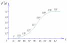 |
For graphic representation of variational series, polygon, histogram, cumulative curve and empirical distribution function are most often used.
In table. 2.3 (Grouping of the population of Russia according to the size of the average per capita income in April 1994) is presented interval variation series.
It is convenient to analyze the distribution series using a graphical representation, which also makes it possible to judge the shape of the distribution. A visual representation of the nature of the change in the frequencies of the variational series is given by polygon and histogram.
The polygon is used when displaying discrete variational series.
Let us depict, for example, graphically the distribution of housing stock by type of apartments (Table 2.10).
Table 2.10 - Distribution of the housing stock of the urban area by type of apartments (conditional figures).

Rice. Housing distribution polygon
On the y-axis, not only the values of frequencies, but also the frequencies of the variation series can be plotted.
The histogram is taken to display the interval variation series. When constructing a histogram, the values of the intervals are plotted on the abscissa axis, and the frequencies are depicted by rectangles built on the corresponding intervals. The height of the columns in the case of equal intervals should be proportional to the frequencies. A histogram is a graph in which a series is shown as bars adjacent to each other.
Let's graphically depict the interval distribution series given in Table. 2.11.
Table 2.11 - Distribution of families by the size of living space per person (conditional figures).
| N p / p | Groups of families by the size of living space per person | Number of families with a given size of living space | Accumulated number of families |
| 1 | 3 – 5 | 10 | 10 |
| 2 | 5 – 7 | 20 | 30 |
| 3 | 7 – 9 | 40 | 70 |
| 4 | 9 – 11 | 30 | 100 |
| 5 | 11 – 13 | 15 | 115 |
| TOTAL | 115 | ---- | |

Rice. 2.2. Histogram of the distribution of families by the size of living space per person
Using the data of the accumulated series (Table 2.11), we construct distribution cumulative.

Rice. 2.3. The cumulative distribution of families by the size of living space per person
The representation of a variational series in the form of a cumulate is especially effective for variational series, the frequencies of which are expressed as fractions or percentages of the sum of the frequencies of the series.
If we change the axes in the graphic representation of the variational series in the form of a cumulate, then we get ogivu. On fig. 2.4 shows an ogive built on the basis of the data in Table. 2.11.
A histogram can be converted to a distribution polygon by finding the midpoints of the sides of the rectangles and then connecting these points with straight lines. The resulting distribution polygon is shown in fig. 2.2 dotted line.
When constructing a histogram of the distribution of a variational series with unequal intervals, along the ordinate axis, not the frequencies are plotted, but the distribution density of the feature in the corresponding intervals.
The distribution density is the frequency calculated per unit interval width, i.e. how many units in each group are per unit interval value. An example of calculating the distribution density is presented in Table. 2.12.
Table 2.12 - Distribution of enterprises by the number of employees (figures are conditional)
| N p / p | Groups of enterprises by the number of employees, pers. | Number of enterprises | Interval size, pers. | Distribution density |
| A | 1 | 2 | 3=1/2 | |
| 1 | up to 20 | 15 | 20 | 0,75 |
| 2 | 20 – 80 | 27 | 60 | 0,25 |
| 3 | 80 – 150 | 35 | 70 | 0,5 |
| 4 | 150 – 300 | 60 | 150 | 0,4 |
| 5 | 300 – 500 | 10 | 200 | 0,05 |
| TOTAL | 147 | ---- | ---- |
For a graphical representation of variation series can also be used cumulative curve. With the help of the cumulate (the curve of the sums), a series of accumulated frequencies is displayed. Accumulated frequencies are determined by sequentially summing the frequencies by groups and show how many units of the population have feature values no greater than the considered value.

Rice. 2.4. Ogiva distribution of families according to the size of living space per person
When constructing the cumulate of an interval variation series, the variants of the series are plotted along the abscissa axis, and the accumulated frequencies along the ordinate axis.
Continuous variation series
A continuous variational series is a series built on the basis of a quantitative statistical sign. Example. The average duration of diseases of convicts (days per person) in the autumn-winter period in the current year was:| 7,0 | 6,0 | 5,9 | 9,4 | 6,5 | 7,3 | 7,6 | 9,3 | 5,8 | 7,2 |
| 7,1 | 8,3 | 7,5 | 6,8 | 7,1 | 9,2 | 6,1 | 8,5 | 7,4 | 7,8 |
| 10,2 | 9,4 | 8,8 | 8,3 | 7,9 | 9,2 | 8,9 | 9,0 | 8,7 | 8,5 |